Stochastic light curves: Orstein-Uhlenbeck process.
We are going to implement and analyze the Orstein-Uhlenbeck process and its implementation in the context of Monte Carlo generation of synthetic light curves for *MUTIS*.
Wiener process, a.k.a one of the simplest SDE:
\[dX = f (X, t)dt + f(X, t)dW_t\]
One of the simplest form it can take is
\[ \begin{align}\begin{aligned}dX = θ (μ − X)dt + σ XdW_t\\a.k.a the Orstein-Uhlenbeck process.\end{aligned}\end{align} \]
[1]:
import numpy as np
import scipy as sp
import scipy.integrate
import scipy.stats
import scipy.signal
import pandas as pd

import matplotlib as mplt
import matplotlib.pyplot as plt

from matplotlib.offsetbox import AnchoredText

from numpy import pi as pi

#%matplotlib widget
Set up parameters
Define the parameters of the process and its precision on integration.
[2]:
theta = 0.1
mu = 0.5
sigma = 0.8
X0 = mu

N = 10000
tf = 200

l = 2*theta/sigma**2
l
[2]:
0.31249999999999994
Integrate
Using scipy integrator
[3]:
%%time
# Integrator 1
dt = tf/N

def yp(t,y):
    return theta*(mu-y)+sigma*y*np.random.randn()/np.sqrt(dt)

t = np.linspace(0,tf,N)

sol = sp.integrate.solve_ivp(yp, y0=[X0], t_span=(0,tf), t_eval=t)
CPU times: user 16 s, sys: 232 ms, total: 16.2 s
Wall time: 15.9 s
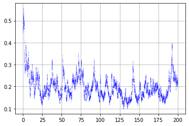
[4]:
plt.figure()
plt.plot(sol.t,sol.y[0], 'b.--', lw=0.1, markersize=0.2)
plt.grid()
plt.show()
Just integrate the fuck out of it
[5]:
%%time

# Integrator 2
t = np.linspace(0,tf,N)
y = np.empty(N)

y[0] = X0
for i in np.arange(1,N):
    y[i] = y[i-1] + dt*(theta*(mu-y[i-1]) + sigma*y[i-1]*np.random.randn()/np.sqrt(dt))
CPU times: user 28.1 ms, sys: 0 ns, total: 28.1 ms
Wall time: 27.8 ms
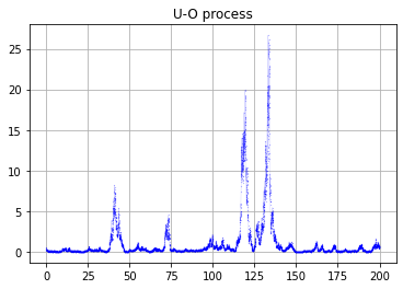
[6]:
plt.figure()
plt.title('U-O process')
plt.plot(t,y, 'b.--', lw=0.1, markersize=0.2)
#plt.ylim([0,3])
plt.grid()
plt.show()
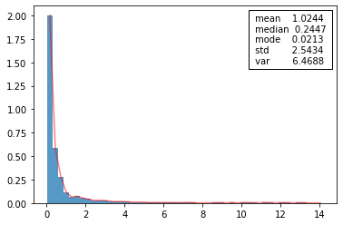
Compare distributions
[7]:
bins = int(y.size**0.5/1.5) #bins='auto'
rang = (np.percentile(y,0), np.percentile(y,99))

fig, ax = plt.subplots()
ax.hist(y, density=True, color='b', alpha=0.4, bins=bins, range=rang)


ax2 = ax.twinx()
y2 = sol.y[0]

bins = int(y2.size**0.5/1.5) #bins='auto'
rang = (np.percentile(y2,0), np.percentile(y2,99))
plt.hist(y2, density=True, color='r', alpha=0.4, bins=bins, range=rang)
plt.show()

Statistical analysis of the generated curve
Plot distribution and fit psd curve
[8]:
bins = int(y.size**0.5/2) #bins='auto'
rang = (np.percentile(y,0), np.percentile(y,99))

p, x = np.histogram(y, density=True, bins=bins, range=rang) #bins='sqrt')
x = (x + np.roll(x, -1))[:-1] / 2.0
[9]:
%%time

plt.figure()

plt.hist(y, density=True, alpha=0.75, bins=bins, range=rang)
plt.plot(x,p,'r-', alpha=0.5)

anchored_text = AnchoredText(" mean    {:.4f} \n median  {:.4f} \n mode    {:.4f} \n std        {:.4f} \n var        {:.4f}".format(np.mean(y), np.median(y), sp.stats.mode(y)[0][0], np.std(y), np.var(y)), loc='upper right')
plt.gca().add_artist(anchored_text)


pdf = lambda x,l,mu: (l*mu)**(1+l)/sp.special.gamma(1+l)*np.exp(-l*mu/x)/x**(l+2)

try:
    popt, pcov = sp.optimize.curve_fit(f=pdf, xdata=x, ydata=p)
    x_c = np.linspace(0,1.1*np.max(x),1000)
    plt.plot(x_c,pdf(x_c,*popt), 'k--')

    print('popt: ')
    print(popt)
    print('pcov: ')
    print(np.sqrt(np.diag(pcov)))

    l_est, mu_est = popt
    eps = 0.05*mu_est
    idx = np.abs(y-mu_est) < eps

    dy = y[1:]-y[:-1]
    sig_est = 1/(np.std(dy[idx[:-1]])/np.sqrt(dt))
    print('sig_est: (método chusco)')
    print(sig_est)

except Exception as e:
    print('Some error fitting:')
    print(e)

plt.show()
Some error fitting:
Optimal parameters not found: Number of calls to function has reached maxfev = 600.
/home/docs/checkouts/readthedocs.org/user_builds/mutis/envs/dev/lib/python3.7/site-packages/ipykernel_launcher.py:10: RuntimeWarning: invalid value encountered in double_scalars
  # Remove the CWD from sys.path while we load stuff.
CPU times: user 274 ms, sys: 52.5 ms, total: 326 ms
Wall time: 236 ms
Extraction of sigma
[10]:
dy = y[1:]-y[:-1]
sigma_est = (np.mean(dy**2/y[:-1]**2))**0.5/np.sqrt(dt)
sigma_est
[10]:
0.7991454734139739
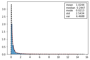
Fit data to distribution with MLE
[11]:
%%time

plt.figure()

plt.hist(y, density=True, alpha=0.75, bins=bins, range=rang)
plt.plot(x,p,'r-', alpha=0.5)

anchored_text = AnchoredText(" mean    {:.4f} \n median  {:.4f} \n mode    {:.4f} \n std        {:.4f} \n var        {:.4f}".format(np.mean(y), np.median(y), sp.stats.mode(y)[0][0], np.std(y), np.var(y)), loc='upper right')
plt.gca().add_artist(anchored_text)


class OU(sp.stats.rv_continuous):
    def _pdf(self,x,l,mu):
        return (l*mu)**(1+l)/sp.special.gamma(1+l)*np.exp(-l*mu/x)/x**(l+2)
try:
    fit = OU(a=0.00001, b=100*np.percentile(y,100)).fit(y,1,1, floc=0, fscale=1)

    print('fit: ')
    print(fit)

    x_c = np.linspace(0,1.1*np.max(x),1000)
    plt.plot(x_c,pdf(x_c, fit[0],fit[1]), 'k--')
except Exception as e:
    print('Some error fitting:')
    print(e)

plt.show()
fit:
(0.0028528911863562097, 57.04810973594368, 0, 1)
/home/docs/checkouts/readthedocs.org/user_builds/mutis/envs/dev/lib/python3.7/site-packages/ipykernel_launcher.py:10: RuntimeWarning: divide by zero encountered in true_divide
  # Remove the CWD from sys.path while we load stuff.
/home/docs/checkouts/readthedocs.org/user_builds/mutis/envs/dev/lib/python3.7/site-packages/ipykernel_launcher.py:10: RuntimeWarning: invalid value encountered in true_divide
  # Remove the CWD from sys.path while we load stuff.
CPU times: user 35.6 s, sys: 80 ms, total: 35.7 s
Wall time: 35.5 s
[12]:
fit[0]*sigma_est**2/2
[12]:
0.0009109759241543101
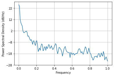
PSD analysis
[13]:
def curvestats(x):
     return pd.DataFrame({'mean':np.mean(x), 'median':np.median(x), 'mode':sp.stats.mode(x)[0][0], 'gmean':sp.stats.gmean(x),
                          'std':np.std(x), 'var':np.var(x),
                          'mM/2':(np.amin(y)+np.amax(y))/2,
                          '0.95mM/2':(np.percentile(x,5)+np.percentile(x,95))/2}, index=[0])
[14]:
sig = y
t = t

plt.figure()

plt.psd(sig.real)

plt.show()
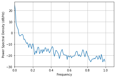
[15]:
plt.figure()

fft = np.fft.fft(sig);
fftp = fft+3*np.random.randn(fft.size);
sigp = np.fft.ifft(fftp);


plt.psd(sigp)
plt.xlim([0,plt.gca().get_xlim()[-1]])

plt.show()
[16]:
sig = y


f, Pxx = sp.signal.welch(sig)
#fft2 = np.sqrt(2*Pxx*Pxx.size)*np.exp(1j*2*pi*np.random.randn(Pxx.size))
fft2 = np.sqrt(2*Pxx*Pxx.size)*np.exp(1j*2*pi*np.random.random(Pxx.size))
sig2 = np.fft.irfft(fft2, n=sig.size)
a = (sig.std()/sig2.std())
b = sig.mean()-a*sig2.mean()
sig2 = a*sig2+b


fftpp = fft
sigpp = sig2
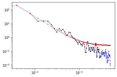
[17]:
plt.figure()

plt.plot(f,Pxx, 'b.-', lw=0.5, markersize=3, alpha=0.8)
plt.xscale('log')
plt.yscale('log')

S = lambda w,b,a,c: a/w**b+c
msk = np.logical_and(0.005 < f,  f < 0.3)
popt, pcov = sp.optimize.curve_fit(f=S,xdata=f[msk],ydata=Pxx[msk],p0=(1.0,1,0))

print('popt:')
print(popt)

print('pcov:')
print(np.sqrt(np.diag(pcov)))

b, a, c = popt

plt.plot(f[msk],Pxx[msk], 'k.-', lw=0.5, markersize=3, alpha=0.8)
plt.plot(f,a/f**b+c,'r.--', lw=0.5, markersize=3, alpha=0.8)

plt.show()
popt:
[2.01121953 0.00307646 0.25225852]
pcov:
[0.09146433 0.00133795 0.19735316]
/home/docs/checkouts/readthedocs.org/user_builds/mutis/envs/dev/lib/python3.7/site-packages/ipykernel_launcher.py:20: RuntimeWarning: divide by zero encountered in true_divide
[ ]: